
Home |
Tutorial |
Theory |
References |
ENM 1.0 |
ANM 2.0 |
Computational & Systems Biology |
NTHU site
|
|
|
Home |
Tutorial |
Theory |
References |
ENM 1.0 |
ANM 2.0 |
Computational & Systems Biology |
NTHU site
|
Theory
GAUSSIAN NETWORK MODEL (GNM)
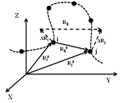
Figure 1: Schematic representation of equilibrium position vectors of residues, their distance vectors and fluctuations.
The GNM is based on the statistical mechanical theory developed by Flory and coworkers for polymer gels (1), where network junctions undergo Gaussian fluctuations. In the GNM, the positions of the network junctions/nodes are identified with the Ca atoms, and the elastic springs represent the interactions that stabilize the native contacts. Two residues are assumed to be in contact when their a-carbons are separated by less than a cutoff distance Rc, which is usually taken around 7 Å. As shown schematically in Figure 1, the fluctuation in the distance between the ith and jth residues is denoted as
|
ΔRij = Rij - Rij0 = ΔRj – ΔRi |
(1) |
where Rij is the instantaneous distance vector, Rij0 is its equilibrium value and ΔRi = Ri - Ri0 designates the fluctuation in the position vector of residue i. The GNM potential is given by
|
(2) |
Here G is the Kirchhoff matrix, the off-diagonal elements of which are defined as
|
Γij = -1 if Rij ≤ Rc Γij = 0 if Rij > Rc |
(3) |
and the diagonal elements are
|
Γii = - Σj Γij |
(4) |
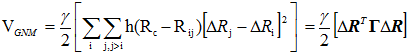
where the summation is performed over all off-diagonal elements in the ith row (or column); h(x) is the Heaviside step function equal to 1 if the argument is positive, zero otherwise; ΔR is an N-dimensional vector composed of the fluctuations of the N-residues.
The cross-correlations between residue fluctuations are found from the statistical mechanical average

|
(5) |
where Γ-1ij is the ijth element of the pseudoinverse of Γ, V is the GNM potential given by Eq. 2. Therefore the evaluation of cross-correlations reduces to that of the ijth element of the inverse of Γ.
The determinant of Γ is 0, and hence Γ-1 cannot be calculated directly. Instead, it is found from the eigenvalue decomposition Γ = ULUT which results in an ensemble of N-1 independent modes. U is the orthogonal matrix whose kth column uk is the kth eigenvector of Γ, and L is the diagonal matrix of eigenvalues lk which are usually organized in ascending order. One of the eigenvalues is identically zero, and the remaining N-1 eigenvalues define each the frequency of the N-1 GNM modes. The ith element (uk)i of uk describes the motion of the ith residue along the kth normal mode coordinate; or, the elements of the kth eigenvector uk represent the distribution of residue displacements (normalized over all residues) along the kth mode axis, and the corresponding eigenvalue lk scales with the frequency of the mode. The size of the motion along the kth mode scales with (1/lk)1/2. Thus (1/lk)1/2 serves as the ‘weight’ of a displacement along mode k. Clearly the lowest frequency modes (small lk) also called slowest modes or softest modes make the largest contribution to the overall motion.
The cross-correlation between residues can be written as a sum of N-1 GNM modes as
|
|
(6) |
The mean-square fluctuations of residue i in mode k can be evaluated from Eq. 6 by replacing j by i. The plot of tr[uk ukT] as a function of residue i represents the probability distribution of residue square fluctuations in mode k, also called kth mode profile.
The cross-correlations are usually shown in a matrix/map format, with the diagonal terms representing the mean-square fluctuations. This ijth element of this matrix, termed cross-correlation matrix, is
|
Cij = < ΔRi . ΔRj > |
(7) |
The normalized cross-correlations are given by
|
Cij (n) = < ΔRi . ΔRj > / [< ΔRi . ΔRi > < ΔRj . ΔRj >]1/2 |
(8) |
Cij (n) varies in the range [-1, 1] and provides information on orientational correlations between the motions of residues i and j. For more information see references (2-7) listed below.
Degree of collectivity
The degree of collectivity of a given mode measures the extent to which the structural elements move together in that particular mode. A high degree of collectivity means a highly cooperative mode, that engages a large portion of (if not the entire) structure. Conversely, low collectivity refers to modes that affect small/local regions only. Modes of high degree of collectivity are generally of interest as functionally relevant modes. These are usually found at the low frequency end of the mode spectrum.
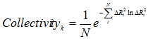
Collectivity for a given mode k is a measure of the degree of cooperativity (between residues) in that mode, defined as (8,9)
|
(9) |
where, k is the mode number, and i is the residue index.
References
1. Flory,P. (1976) Statistical thermodynamics of random networks. Proc. R. Soc. Lond. A, 351, 351-380.
2. Bahar,I., Atilgan,A.R. and Erman,B. (1997) Direct evaluation of thermal fluctuations in proteins using a single-parameter harmonic potential. Fold. Des., 2, 173-181.
3. Bahar,I., Atilgan,A.R., Demirel,M.C. and Erman,B. (1998) Vibrational Dynamics of Folded Proteins: Significance of Slow and Fast Motions in Relation to Function and Stability. Phys. Rev. Lett., 80, 23.
4. Bahar,I. and Rader,A.J. (2005) Coarse-grained normal mode analysis in structural biology. Curr. Opin. Struct. Biol., 15, 586-592.
5. Rader,A.J., Chennubhotla,C., Yang,L.W. and Bahar,I. (2006) The Gaussian network model: Theory and applications. In Bahar,I. and Cui,Q. (eds.), NORMAL MODE ANALYSIS: THEORY AND APPLICATIONS TO BIOLOGICAL AND CHEMICAL SYSTEMS. Chapman & Hall/CRC: Boca Raton, FL, pp. 41-64.
6. Eyal,E., Dutta,A. and Bahar,I. (2011) Cooperative dynamics of proteins unraveled by network models. WIREs Comput Mol Sci, 1, 426-439.
7. Yang,L.W. (2011) Models with energy penalty on interresidue rotation address insufficiencies of conventional elastic network models. Biophys. J., 100, 1784-1793.
8. Tama,F. and Sanejouand,Y.H. (2001) Conformational change of proteins arising from normal mode calculations. Protein Eng., 14, 1-6.
9. Brüschweiler,R. (1995) Collective protein dynamics and nuclear spin relaxation. J. Chem. Phys., 102, 3396-3403.